Power calculations
Summary
This section is intended to provide an intuitive discussion of the rationale behind power calculations, as well as practical tips and sample code for conducting power calculations using either built-in commands or simulation. It assumes some knowledge of statistics and hypothesis testing. Readers interested in more technical discussions may refer to the links at the bottom of the page, those looking for sample code for conducting power calculations in Stata or R may refer to our GitHub page, and those looking for an intuitive tool to engage with power calculations for teaching purposes or to engage with partners may refer to our power calculator (also linked in the "Sample code and calculator" section below). Those already familiar with the intuition and technical aspects may refer to our Quick guide to power calculations.
Essentials
- The sensitivity of an experiment to detect differences between the treatment and the control groups is measured by statistical power.
- A type I error is a false positive: falsely rejecting the null hypothesis of no effect, or falsely concluding that the intervention had an effect when it did not. The probability of committing type I error is known as α.
- A type II error is a false negative: failing to detect an effect when there is one. The probability of committing type II error is typically given by β. To differentiate it from the treatment effect β, in this resource we denote type II errors by κ.
- Power is the probability of rejecting a false null hypothesis. Formally, power is typically given by 1-β. Again, to differentiate power from the treatment effect β, in this resource we will denote power by 1-κ. That is, maximizing statistical power is to minimize the likelihood of committing a type II error.
- Power calculations involve either determining the sample size needed to detect the minimum detectable effect (MDE) given other parameters, or determining the effect size that can be detected given a set sample size and other parameters.
Components of power calculations include:
- Significance (α): The probability of committing a type I error. It is typically set at 5%, i.e., α=0.05.
- Power (1-κ): Typically set at 0.8, meaning the probability of falsely failing to reject the null hypothesis is 0.2 or 20%. Power mirrors the significance level, α: as α increases (e.g., from 1% to 5%), the probability of rejecting the null hypothesis increases, which translates to a more powerful test.
- Minimum detectable effect (MDE): The smallest effect that, if true, has (1-β)% chance of producing an estimate that is statistically significant at the α% level (Bloom 1995). In other words, the MDE is the effect size below which we may not be able to distinguish that the effect is different from zero, even if it is.
- Sample size (N)
- Variance of outcome variable (σ2)
- Treatment allocation (P), the proportion of the sample assigned to the treatment group. Power is typically maximized with an equal split between treatment arms, though there are instances when an unequal split may be preferred.
- Intra-cluster correlation coefficient (ICC): A measure of the correlation between observations within the same cluster, also often given as ρ. If the study involves clustered randomization (i.e., when each unit of randomization contains multiple units of observation), you will need to account for the fact that individuals (or households, etc.) within a group such as a town/village/school are more similar to each other than those in different groups.1 In general, this will increase the required sample size.
Power is also affected by the design of the evaluation, the take up of the treatment, and the attrition rate, discussed in greater detail below.
| Component | Relationship to power | Relationship to MDE |
| Sample size (N) increase | Increases power | Decreases the MDE |
| Outcome variance decrease | Increases power | Decreases the MDE |
| True effect size increases | Increases power | n/a |
| Equal treatment allocation (P) | Increases power | Decreases the MDE |
| ICC increases | Decreases power | Increases the MDE |
Introduction
Hypothesis tests focus on the probability of a type I error, or falsely rejecting the null hypothesis of β=0, i.e., falsely concluding that there is a treatment effect when one does not exist. As written above, significance levels are typically set at 5%, but in taking this conservative approach we increase the risk of a different error: failing to detect a treatment effect when one exists, i.e., a type II error.2 Power is defined as the probability of NOT committing a type II error. That is, power is correctly rejecting the null hypothesis when a treatment effect exists, or [1-prob(type II error)].
The graph below depicts how a type II error could happen:
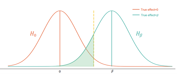
In figure 1, the orange curve is the distribution of $\hat{\beta}$ under the null hypothesis. The teal curve is the distribution of $\hat{\beta}$ under the alternative hypothesis. The green shaded region comprises 20% of the area under the curve. If the true effect is $\beta$, the green shaded region is the probability of failing to reject the null hypothesis even though the alternative hypothesis is true.
Randomization at the unit of observation
Power and sample size equations
There are two main approaches to calculating power, depending on whether the study’s sample size is fixed:
-
If the sample size is fixed according to budget constraints or external factors (e.g., the number of eligible children in a partner’s schools), power calculations determine the effect size the study is powered to detect (the MDE). Researchers then decide whether the study should go forward as designed or whether the design should be tweaked to increase power. Formally3:
- If the sample size is not fixed or capped at a predetermined number, power calculations can be performed to determine the minimum sample size needed to detect an effect size (the MDE) given the parameters:
Where, as defined above, N denotes the sample size, $\sigma^2$ the outcome variance (which is assumed to be equal in each treatment arm), P the treatment allocation, and $t_{1-\kappa}$ and $t_{\frac{\alpha}{2}}$ the critical values from a Student’s t distribution for power and significance, respectively. See Liu (2013) for more information on why power calculations use the t distribution instead of a normal distribution.
More complicated designs, such as clustered designs or those that include covariates or strata, will require more information (more below). Details on potential sources for obtaining this information can be found in the section "Practical Tips" for calculating power below.
Relationship between power and power components
The figures and equations presented above provide additional intuition for the relationship between power and its components, holding all else equal. This section discusses this intuition then summarizes the relationships in a table below.
Outcome variance and sample size: Sample outcome variance decreases as sample size increases, as larger samples are more representative of the underlying population. This leads to a more precise treatment effect estimate, which in turn lowers the probability of a type II error and hence increases power. The same is true of outcomes with less variation in the underlying population because sample variance will typically be smaller when the population variance is smaller. Note that this can also be seen analytically using the calculation of standard errors above: as the sample size (N) increases, or as the population variance (𝜎2) decreases, the standard error will decrease.
Figure 2 shows that as the variance of the beta decreases, the null and the alternate hypothesis become narrower, a larger portion of the alternate hypothesis lies to the right of the critical value (critical value represented by the dashed yellow line) and the power increases (teal shading).
True effect size: Figure 3 below provides intuition for how the absolute value of the true effect size affects power. Holding all else equal, as the absolute true effect size increases, the entire distribution of $\hat{\beta}$ under the alternative hypothesis (the teal curve) shifts further away from the distribution of $\hat{\beta}$ under the null hypothesis (the orange curve), while the critical value (the yellow line) remains the same. That is, power increases as the absolute true effect size increases. Intuitively, if the absolute true effect size is higher, the probability of detecting the effect increases.
Treatment allocation: From equation 1, it can be seen that the MDE is minimized with an even split of units between treatment and control, i.e., P=0.5, holding all other parameters fixed. Intuitively, starting with an unequal allocation and adding an additional unit to the smaller group (creating a more even split) reduces sampling variation by more than if the unit were added to the larger group. Since power decreases when MDE decreases, power decreases as the treatment allocation deviates from 0.5. In most cases, of course, all other parameters will not be fixed. Two common situations when a deviation from a 50/50 split is desirable are when there are:
- Budget constraints: If the cost of the intervention is high (as opposed to the cost of data collection, which will be equal across treatment groups), then power subject to the budget constraint may be maximized by a larger control group (both overall and a larger proportion of units assigned to the control group). Per Duflo et al. (2007), the optimal allocation under these circumstances is then: $\frac{P}{1-P}=\sqrt{\frac{c_c}{c_t}}$ (equation 3)
Where $c_c$ and $c_t$ denote the cost per control and treatment unit, respectively. That is, the optimal allocation of treatment to control assignment is proportional to the square root of the inverse of the per unit costs. See section 6 of McConnell and Vera-Hernandez (2015) for a discussion on treatment allocation under cost constraints.
- Concerns about withholding a program which is thought to be effective: If a program is thought to be effective but still warrants evaluating (e.g., for cost-effectiveness comparisons with similar programs), options include 1) a larger treatment group or 2) an encouragement design, where the entire eligible population has access to the program, but only the treatment group receives encouragements to take it up. See more in J-PAL North America’s Real-world challenges to randomization and their solutions.
- Different standard deviations between the treatment and control groups after the treatment: Unequal treatment allocation will yield more power if we expect that the treatment will have an effect on the variance of the outcome variable. The optimal sample split is the ratio of the variance of the treatment and the control groups. The group with the larger variance should be allocated a greater proportion of the sample. Refer to McConnell and Vera-Hernandez (2015) and Özler (2021) for a discussion on the statistical framework and practical calculations of power with unequal variances.
Take-up, noncompliance, and attrition: Noncompliance effectively dilutes the treatment effect estimate, with either the treatment group including units that were not treated, the control group including units that were, or both. This requires a larger sample size to detect the MDE. Again using the notation of Duflo et al. (2007) on page 33 of the randomization toolkit, $c$ denotes the share of treatment group units that receive the treatment and $s$ the share of control group units receiving the treatment. Then the MDE is given as follows:
Equation 4: $$ MDE=(t_{1-\kappa}+t_{\frac{\alpha}{2}})\sqrt{\frac{1}{P(1-P)} \times \frac{\sigma^2}{N}} \times \frac{1}{c-s} $$With incomplete take-up or noncompliance the necessary sample size is inversely proportional to $(c-s)$, i.e., the difference in take-up between the treatment and control groups. For example, if only half of the treatment group takes up the treatment, while no one in the control group does (i.e., $c-s=0.5$), and holding all else equal, the necessary sample size to detect a given effect size would be four times larger than with perfect compliance.
Attrition can also reduce power (or, conversely, increase the MDE) since the study sample is smaller than previously intended. Different attrition rates between the treatment and the control can also move the allocation ratio closer or farther away from the original allocation. Rickles et al. (2019) discuss how different types of attrition (random, conditional on treatment assignment or conditional on covariates) can affect the MDE.
Relationship between the MDE and power components: Conceptually, the components listed above affect the MDE in a similar manner as they do power, summarized in table 1 above.
Clustered designs
The power calculations presented so far are for randomization at the same unit of observation. Clustered randomization designs, in which each unit of randomization contains multiple units of observation, require modifications to the power calculation equations. Examples of clustered designs include randomizing households but measuring individual-level outcomes or randomizing health clinics and measuring patient-level outcomes.
Intracluster correlation coefficient
The correlation between units within a cluster is given by the intracluster correlation coefficient (ICC). Formally, it is the fraction of total variation in the outcome variable that comes from between-cluster variation (Gelman and Hill 2006):
Equation 5:$ICC = \frac{\sigma^2_{between-cluster}}{\sigma^2_{between-cluster}+\sigma^2_{within-cluster}}$
Where the denominator in the above equation is the total variation of the outcome variable, decomposed into the sum the within-cluster variation ($\sigma^2_{within-cluster}$) and between-cluster variation ($\sigma^2_{between-cluster}$). The ICC ranges from 0 to 1 and is often denoted by $\rho$.
If individuals within clusters were identical to each other (e.g., if all members of a household voted the exact same way), then the variation in the sample would be driven entirely by differences between clusters rather than differences between individuals within a cluster. In this case, the ICC would equal 1 and the effective sample size would be the number of clusters. If, on the other hand, individuals within clusters were completely independent of each other, the ICC would equal 0. In this instance, the effective sample size would be the number of individuals.
In practice, the ICC is typically somewhere between 0 and 1, meaning that the effective sample size is greater than the number of clusters but smaller than the number of individual units. The actual size of the ICC will depend on the degree of similarity between units within a cluster, with the ICC increasing (and effective sample size decreasing) if units within the cluster behave more similarly to each other. This decrease in effective sample size, in turn, reduces precision and increases the MDE. Suggestions for calculating the ICC are provided in the section "Practical Tips" for calculating power below.
Power equations for clustered designs
As mentioned above, in clustered designs the total sample size $N$ can be split into the number of clusters $k$ and the average number of units per cluster $m$. To adjust for correlation within clusters, power calculations in clustered designs include the design effect, which is given by $(1+(m-1) \times ICC)$. The equation for the MDE in a clustered design is then given by:
Equation 6: $$ MDE = (t_{1-\kappa}+t_{\frac{\alpha}{2}} \sqrt{\frac{1}{P(1-P)} \times \frac{\sigma^2}{N} \times (1+(m-1)\times ICC)} $$With the exception of $N$ (for the reasons described above), the components of this equation affect the MDE in a manner similar to the way described above for an individual-level randomization. Note here how an increase in the ICC inflates the MDE or required sample size. For example, holding $N$ and $P$ fixed, setting $m=50$, and an ICC of 0.07, the standard error of the treatment effect estimator (the square root term) doubles. As a result, the MDE doubles, while the required sample size quadruples.
Practical tips
This section provides an overview of sources for each component of power calculations and tips for running initial calculations. It also covers guidance on refining calculations based on interest in binary or multiple outcomes and design features such as unequal cluster size or stratified randomization.
Gathering inputs
Some components of power calculations are based on decisions or assumptions made by the researcher and partner, while others are calculated using existing data.
Based on decisions or assumptions:
-
Power (1-κ) is typically set at 80%, or 0.8, though in some cases it is instead set at 90%. While it can be tempting to increase a study’s power, doing so also increases the risk of a false positive (type I error). See Cohen (1988) for more information.
- Significance level (α) is typically set at 5%, i.e., α=0.05.
- Units of randomization and observation: The units of randomization and observation do not need to be the same. See the “Implementation” section of the Randomization resource for more information on determining each. In clustered designs, while the addition of more clusters will in general increase power more than the addition of more units to existing clusters, the former is typically more expensive to do.
- MDE may be a practically relevant effect size such as the minimum improvement in outcomes required for the implementing partner to determine the program’s benefits are worth the costs or to scale the program. Note that published studies evaluating similar interventions will typically provide an optimistic estimate of a reasonable effect size. This difference will be diluted by any non-compliance, so the expected effect size should be adjusted to the expected compliance rate in the two groups.
- If information about realistic effect sizes is not available, Cohen (1988) proposes rules of thumb that rely on standard deviations4: 0.2 standard deviations for a small MDE, 0.5 standard deviations for a medium MDE, and 0.8 standard deviations for a large MDE. These standards are based on social psychology lab experiments among undergraduates, however, and have since been argued not to be realistic in real-world settings for some sectors and regions--see e.g., Kraft (2019) (associated blog post) and Evans and Yuan (2020) (associated blog post) for discussions of why smaller MDEs may be more realistic for education interventions.
- Alternatively, the sample size (N) may be determined by the study budget or a partner’s constraints (e.g., number of eligible students in the partner’s schools, the number of health clinics in the district, etc.).
- Number of clusters (k) and size of each cluster (m): It is typically cheaper to interview one more person in an existing cluster than add a new cluster due to logistical constraints (transportation, personnel costs etc.). However, the marginal cost decrease from one additional unit in an existing cluster should be weighed against the decreasing marginal power from each additional unit. The optimal number of clusters and the size of each cluster will also change based on the expected ICC.
- Treatment allocation (P) can be manipulated to maximize power or to minimize costs. As written above, power is typically maximized with an equal allocation of units to treatment and control groups, but it is costlier to provide the treatment to more units. As a result, it’s possible that an unequal treatment allocation (e.g., 30% treatment 70% control) with a larger total sample size will be better powered than a 50/50 split with a smaller sample size. It is worth testing different sample sizes and treatment allocations given budget constraints to find the design that maximizes power. See chapter 6 of Running Randomized Evaluations for a guide on adjusting the allocation ratio to different practical scenarios.
Calculated using data such as from a baseline or pilot, existing studies, or publicly available data:
-
Outcome variance (σ2) is ideally found in baseline data. If that is not available, it may be calculated using other data in the same or a similar population, or found in papers from studies on similar topics, preferably among similar populations. Useful data sources include the J-PAL/IPA Dataverses, administrative data, LSMS data, etc.5 Note that it is typically assumed that the outcome variance is the same across treatment arms.
-
ICC: Similarly, the ICC can be estimated using data from baseline data, surveys, and papers--all preferably in the same or a similar population. See McKenzie (2012) for an explanation of one of the ways to calculate ICC based on baseline data in Stata.
- Take-up, compliance, and attrition: Literature from previous programs similar to the one under study can give a rough idea of plausible levels of take-up. Note that such literature need not be restricted to academic papers but can also include white and gray literature, reports, etc.
Initial calculations
Initial calculations should focus on whether the study may be feasible. After a proposed project passes a basic test of feasibility, power calculations can be refined and updated with new data. In performing initial calculations, keep the following in mind:
- Run initial calculations with the best data that is readily accessible, and avoid getting bogged down seeking access to non-public data or sorting out details that can be adjusted.
- You may not need to find data for each component to run power calculations. From sensitivity analysis (below) you will learn which inputs have the largest impact on power. Focus the team’s efforts on finding good estimates for the inputs that matter most.
- Similarly, if you are missing information on certain power components, make reasonable assumptions to check potential feasibility of the study. For example, use the rules of thumb for effect sizes listed above: a 0.2 standard deviation increase is a small effect size; use this as a starting MDE and calculate the necessary sample size to determine basic feasibility.
- Perform sensitivity analysis to test how power changes with changes to any critical assumptions. Focus particularly on:
- Key assumptions such as minimum effect size, take-up rates and intracluster correlation. Be realistic and, if anything, overly pessimistic about take-up rates.
- Any information that was assumed due to missing data (e.g., effect sizes as in the bullet above).
- Areas where there is some leeway for adjusting the design, such as adding units to clusters instead of vice versa, shifting treatment allocations, etc.
- Consider both analytical and simulation methods. Simulated calculations are especially helpful for more complex study designs (McConnell and Vera-Hernandez, 2015). They involve: 1) creating a fake dataset with a pre-determined effect size and design features, 2) testing the null hypothesis, 3) repeating steps 1 and 2 many (usually 1,000 or more) times, and 4) dividing the total number of rejections from step 2 by the total number of tests to calculate power. With good data on the study population, they can also be used to calculate simulated confidence intervals around null effects, or in power calculations for a small sample where some of the parametric assumptions about probability distributions may not hold. Sample code for both approaches can be found on our GitHub.
Refining calculations
If the study looks promising based on initial calculation, the next steps are to iterate over details of the study design and refine calculations to get a more precise estimate of the necessary sample size. Note that refinements may be minimal or not even necessary at all. For example, there may be no need to iterate further if the sample size is fixed and initial calculations made with reliable and relevant data showed that the design is powered under a wide range of assumptions about the ICC, take-up, etc. On the other hand, there are two key assumptions where refinements may be particularly helpful:
-
Significant changes in design from what was assumed in initial calculations—such as changing the number of treatment arms, changing intake processes (which might affect take-up), changing the unit of randomization, or deciding you need to detect effects on particular subgroups—should inform, and be informed by, estimates of statistical power.
-
Better estimates of key inputs: If the study has passed a basic feasibility test but there were first-order inputs for which you were unable to find satisfactory estimates for initial power calculations, it may be worth seeking additional data to refine power estimates. Consider requesting detailed operational data from the partner, or requesting non-public survey or administrative data from a third party.
If not included in initial calculations, there are additional design factors to consider when refining calculations, described further below.
Additional design factors to consider
For more information about the underlying theory of how design choices, interest in different kinds of effects, or the use of binary outcome variables influence power calculations, see McConnell and Vera-Hernandez (2015), Athey and Imbens (2017), Duflo et al. (2007), or Baird et al. (2018). Tips for incorporating such design decisions into power calculations are described below.
Binary outcomes: The outcome of interest may be a binary variable, such as whether a person is employed after a job-training program, whether a student passed a grade after a tutoring program etc. While the intuition for determining the MDE and sample size is the same as for a continuous variable, the effect size and the variance of the outcome variable changes based on the representation (log odds ratio or difference in probability) and calculation (logistic or linear regression) of the effect. See section 5 of McConnell and Vera-Hernandez (2015) for a statistical representation of power and sample code for a binary outcome variable.
Unequal cluster size: Clusters will often be of unequal sizes due to real-world constraints in splitting units--this can include both an unequal number of clusters in each treatment arm as well as an unequal number of units within clusters. For example, a study randomizing at the teacher level and measuring outcomes at the student level will likely have different size clusters. Unless there is wide variation in cluster sizes, the total sample size required will be only slightly higher with unequal clusters than it would be with equal clusters. See page 12 of McConnell and Vera-Hernandez (2015) for more.
Stratified randomization: Though randomization removes ex ante systematic bias between the treatment and the control groups, researchers may choose to stratify random assignment to ensure that the treatment and the control groups have a similar proportion of units with certain important characteristic(s). Since the stratification variable is likely to be correlated with the outcome variable, stratification will typically reduce the residual variance of the outcome variable, increasing power. See J-PAL's randomization resource and Athey and Imbens (2017) for more information on stratification.
Heterogeneous treatment effects: Stratification can also be useful for calculating the heterogeneous effects of the treatment among certain groups. For example, we may be interested in comparing the heterogeneous results among men versus women, among college-educated vs non-college educated voters, etc. In this case, it is useful to conduct separate power calculations for the two groups to ensure that the study is sufficiently powered to detect the heterogeneous treatment effects of interest.
Adding covariates: Similar logic as with stratification applies here: randomization precludes the necessity of including covariates for unbiased estimates of the treatment effect but doing so may be useful to reduce the residual variance of the outcome variable. All else equal, this increases power, though the extent of this depends on the size of the dataset and the correlation between the covariates and the outcome variable, among other factors.6 See J-PAL's data analysis resource for guidance on including covariates in your analysis and Athey and Imbens (2017) for more.
Multiple treatment arms: If the study design includes multiple arms, we may be interested in pairwise comparisons between the treatment arms or between one treatment arm and the control. Ensure that the study is powered for the smallest MDE among the comparisons that will be made (though this can significantly increase costs if comparing two similar treatments). It can be helpful to first calculate the MDE for each pairwise comparison assuming equal allocation fractions, then recalculate the MDEs after rearranging the samples in different ways to understand which comparisons can be meaningfully made within the budget constraint. Note that if in analysis you will adjust for making multiple comparisons between groups (e.g., control and treatment 1, control and treatment 2, treatments 1 and 2, etc.) you should do the same in power calculations.
Multiple outcomes: As with multiple treatments, if the study will look at multiple outcomes, it is important to ensure that it is powered to detect all outcomes, i.e., pick the sample size and design that is powered to detect the smallest MDE of the outcomes of interest.
Multiple hypotheses: When evaluating multiple hypotheses, it is important to note that significance level or the probability of rejecting the null hypothesis increases with the number of hypotheses. This can be dealt with by adjustments for multiple hypothesis testing (MHT), such as with the Bonferroni or Benjamini Hochberg adjustments. Power may increase or decrease based on the type of adjustment, number of hypotheses and the correlation between the null hypotheses (Porter 2016; McConnell and Vera-Hernandez 2015), but if you will adjust for MHT in analysis it is important to do so in power calculations to ensure the study is adequately powered. See J-PAL’s data analysis resource as well as EGAP’s methods guide and McKenzie (2020) for a longer description of the problem, section 4 of List, Shaikh and Xu (2016) for a demonstration of multiple hypothesis adjustments with multiple treatment arms and heterogenous effects, and pages 29-30 of McConnell and Vera-Hernandez (2015) for a description of applications to power calculations.
Interpreting results and troubleshooting
Interpreting the calculated MDE
For a continuous outcome variable, the minimum effect size is measured in the same units as the outcome variable, unless it is a standardized effect size (i.e., the effect size is divided by the outcome standard deviation). In this case, the MDE is expressed in terms of standard deviations. Mechanically, this is done by rearranging the variance term in equation 1.
If the outcome variable is a binary variable, the effect size may be measured as the difference in the log odds ratio or in the probability of success between the treatment and the control. For the latter, the MDE is expressed in percentage points (e.g., an MDE of .06 is interpreted as a 6 percentage point increase over the control group mean). Note that the built-in Stata command power calculates the latter (probability of success) measure.
It is important to remember that statistical power calculations are based on the underlying sampling distribution of the effect estimate. So even if the study has 80 percent power, there is still a 20 percent chance that you might not detect the effect if the program has an impact. Conversely, an underpowered study may still detect an effect if it is true but with a lower probability. The next section discusses possible adjustments if the study is underpowered.
Troubleshooting: Underpowered designs
If the study is underpowered but may be feasible, try to tweak the design or increase the sample size. Some ideas are listed below.
- If budget is the limiting factor: Consider not doing a baseline (McKenzie 2012), changing the treatment allocation (add units to the control group and reduce the number of units in the treatment group), adding units instead of clusters, simplifying the design (e.g., dropping a treatment arm, limiting pairwise comparisons between similar treatments, etc.). See the discussion starting on page 21 of McConnell and Vera-Hernandez (2015) for a statistical framework and sample simulation code for cost optimization.
- Note that stratification has an ambiguous effect on power. As mentioned above, adding covariates or stratifying increases the precision of treatment effect estimates, thereby reducing the total necessary sample size. However, the sample size required to detect heterogeneous treatment effects by stratum will likely be higher. If limited by budget, it is worth testing how stratification affects the study’s power.
- If sample size is the limiting factor: An obvious option is to simplify the design, say by reducing the number of treatment arms or focusing on a smaller set of the most important primary outcomes. As above, the inclusion of covariates can increase power, though if the sample size is fixed and is the limiting factor, you would unlikely be able to detect heterogeneous treatment effects. An alternative, if not limited by budget, is to increase the number of rounds of data collection (McKenzie 2012).
If the study remains underpowered, even with any feasible design tweaks, then the risks of going forward with the study outweigh the benefits, and you should hold off on moving forward until the sample size can be increased, more data is available, etc. At best, an underpowered study is a waste of money—you won’t be able to determine whether the program is effective. At worst, null results from an underpowered study may be used to justify ending a program if they are conflated with the program itself being ineffective. More on this can be found in J-PAL North America’s guide.
Sample code and calculator
Visit our GitHub page for sample Stata and R code for conducting power calculations using built-in commands and by simulation. For an interactive tool to visualize how the components of power calculations impact a study’s required sample size, see our power calculator.
Last updated August 2021.
These resources are a collaborative effort. If you notice a bug or have a suggestion for additional content, please fill out this form.
We thank William Parienté for helpful comments. Any errors our own.
For example, if your experiment is clustered at the school level and the outcome of interest is test scores, the ICC would be the level of correlation in test scores for children in a given school relative to the overall distribution of test scores of students in all schools.
This conservative approach was endorsed by R. A. Fisher, who felt type I errors were worse than type II. A significance level of 5% and a power level of 80% makes the risk of a type II error four times as likely as a type I error. See his 1925 book, Statistical methods for research workers, for more information.
This formula is a direct result of hypothesis testing; see page 28 of Duflo et al. (2007) to learn more. Note that this formula assumes equal variance across the control and the treatment groups before and after treatment. It also does not account for potential heterogeneity across sub-groups in the sample.
Though, as noted by Duflo et al. (2007), this rule of thumb is less helpful when standard deviations are unknown, standard deviations of outcome variables may be available in baseline or publicly available data even when effect sizes are not.
In the case of a binary outcome variable, the variance is a function of the mean of the variable. For a given binary variable $Y$ which takes values 0 or 1 and has mean $P$, $var(Y) = (1-P) \times $P$. The variance for the control and the treatment groups are likely to be different after the intervention since the treatment mean is likely to change after the intervention.
In the extreme, if there is zero correlation between the included covariates or stratifying variables then their inclusion does not increase precision, i.e., stratification is equivalent to complete randomization (Athey & Imbens 2016).
Additional Resources
McConnell, Brendon, and Marcos Vera-Hernandez. 2015. "Going beyond simple sample size calculations: a practitioner's guide." IFS Working Paper W15/17. https://ifs.org.uk/publications/7844.
Kondylis, Florence, and John Loeser. Power Dashboard: Cash transfer size, nonlinearities, and benchmarking. Associated blog posts: part 1 and part 2.
Rickles, Jordan, Kristina Zeiser, and Benjamin West. 2019. "Accounting for Student Attrition in Power Calculations: Benchmarks and Guidance." Journal of Research on Educational Effectiveness, 11(4): 622-644. https://doi.org/10.1080/19345747.2018.1502384.
Evidence in Governance and Politics (EGAP)'s multiple hypotheses guide.
References
Athey, Susan, and Guido Imbens. 2017. “The Econometrics of Randomized Experiments.” Handbook of Field Experiments, 73-140. doi:10.1016/bs.hefe.2016.10.003.
Baird, Sarah, J. Aislinn Bohren, Craig Mcintosh, and Berk Ozler. 2018. “Optimal Design of Experiments in the Presence of Interference.” The Review of Economics and Statistics, 100(5): 844-860. https://doi.org/10.1162/rest_a_00716
Cohen, Jacob. 1998. Statistical Power Analysis for the Behavioral Sciences. 2nd ed., Routledge: New York, USA. https://doi.org/10.4324/9780203771587.
Duflo, Esther, Rachel Glennerster, and Michael Kremer. 2007. “Using Randomization in Development Economics Research: A Toolkit.” Handbook of Development Economics, 3895-3962. doi:10.1016/s1573-4471(07)04061-2.
Evans, David. "We Need Interventions that Improve Student Learning. But How Big is a Big Impact?" Center for Global Development (blog), August 26, 2019. https://www.cgdev.org/blog/we-need-interventions-improve-student-learning-how-big-big-impact. Last accessed August 3, 2021.
Evans, David, and Fei Yuan. 2020. "How Big Are Effect Sizes in International Education Studies?" Center for Global Development Working Paper 545. https://www.cgdev.org/sites/default/files/how-big-are-effect-sizes-international-education-studies.pdf.
Evans, David, and Fei Yuan. 2020. "How Big Are Effect Sizes in International Education Studies?" Center for Global Development (blog), August 27, 2020. https://www.cgdev.org/blog/how-big-are-impacts-international-education-interventions. Last accessed August 3, 2021.
Fisher, Ronald. 1935. The Design of Experiments. Oliver and Boyd: Edinburgh, UK.
Gelman, Andrew, and Jennifer Hill. 2006. "Sample size and power calculations" in Data Analysis Using Regression and Multilevel/Hierarchical Models, 437-454. Cambridge University Press: Cambridge, UK. https://www.cambridge.org/highereducation/books/data-analysis-using-regression-and-multilevel-hierarchical-models/32A29531C7FD730C3A68951A17C9D983?utm_campaign=shareaholic&utm_medium=copy_link&utm_source=bookmark.
Kraft, Matthew A. 2020. "Interpreting Effect Sizes of Education Interventions." Educational Researcher, 49(4): 241-253. https://doi.org/10.3102/0013189X20912798.
List, John A., Azeem M. Shaikh, and Yang Xu. 2019. "Multiple hypothesis testing in experimental economics." Experimental Economics, 22: 773-793. https://doi.org/10.1007/s10683-018-09597-5.
Liu, Xiaofeng. 2013. Statistical Power Analysis for the Social and Behavioral Sciences: Basic and advanced techniques. Routledge: New York, USA. https://doi.org/10.4324/9780203127698.
McConnell, Brendon, and Marcos Vera-Hernandez. 2015. "Going beyond simple sample size calculations: a practitioner's guide." IFS Working Paper W15/17. https://ifs.org.uk/publications/7844.
McKenzie, David. "An overview of multiple hypothesis testing commands in Stata." World Bank Development Impact (blog), June 1, 2021. https://blogs.worldbank.org/impactevaluations/overview-multiple-hypothesis-testing-commands-stata. Last accessed August 3, 2021.
McKenzie, David. 2012. "Beyond baseline and follow-up: The case for more T in experiments." Journal of Development Economics, 99(2): 210-221. https://openknowledge.worldbank.org/bitstream/handle/10986/3403/WPS5639.pdf?sequence=1&isAllowed=y.
McKenzie, David. "Power Calculations 101: Dealing with Incomplete Take-up." World Bank Development Impact (blog), May 23, 2011. https://blogs.worldbank.org/impactevaluations/power-calculations-101-dealing-with-incomplete-take-up. Last accessed August 3, 2021.
McKenzie, David. "Tools of the Trade: Intra-cluster correlations." World Bank Development Impact (blog), December 02, 2012. https://blogs.worldbank.org/impactevaluations/tools-of-the-trade-intra-cluster-correlations. Last accessed August 3, 2021.
Özler, Berk. "When should you assign more units to a study arm?" World Bank Development Impact (blog), June 21, 2021. https://blogs.worldbank.org/impactevaluations/when-should-you-assign-more-units-study-arm?CID=WBW_AL_BlogNotification_EN_EXT. Last accessed August 3, 2021.
Porter, Kristin E. 2016. "Statistical Power in Evaluations That Investigate Effects on Multiple Outcomes: A Guide for Researchers." MDRC Working Paper. https://www.mdrc.org/sites/default/files/EC%20Methods%20Paper_2016.pdf.
Rickles, Jordan, Kristina Zeiser, and Benjamin West. 2019. "Accounting for Student Attrition in Power Calculations: Benchmarks and Guidance." Journal of Research on Educational Effectiveness, 11(4): 622-644. https://doi.org/10.1080/19345747.2018.1502384.